Gravitational lensing in wave optics

We study gravitational lensing in the thin-lens approximation, which is valid when the length scale over which light is deflected is small as compared to the distances from source to lens or lens to observer. The path integral amplitude, normalized to unity in the absence of a lens, reduces in the small-angle (flat sky) approximation to a two-dimensional Kirchhoff-Fresnel integral

\[\psi(\boldsymbol{y}) = \frac{\Omega}{2\pi i} \int e^{i \Omega \left[{1\over 2}(\boldsymbol{x}-\boldsymbol{y})^2 + \varphi(\boldsymbol{x})\right]} \mathrm{d}\boldsymbol{x}.\]

Here, \(\boldsymbol{y}\) and \(\boldsymbol{x}\) denote the position on the sky and on the lens plane respectively. Both are expressed in units of the Einstein angle for the total lens mass. For gravitational lensing by \(N\) point masses located at \(\boldsymbol{x}_i\), \(i=1,\dots N\) on the sky, the lensing phase takes the form

\[\varphi(\boldsymbol{x}) =- \sum_{i=1}^N f_i \log|\boldsymbol{x} - \boldsymbol{x}_i |\,,\]

with \(f_i\) the mass fractions satisfying \(\sum_{i=1}^N f_i=1\). The normalized intensity is given by the magnitude squared of the amplitude

\[I(\boldsymbol{y}) = | \psi(\boldsymbol{y})|^2.\]

When the wavelength is small compared to the Schwarzchild radius for the lens mass, or when the radiation is incoherent, geometric (ray) optics provides an excellent approximation. However, when these conditions are not fulfilled, the interference pattern must be determined by evaluating the highly oscillatory Kirchhoff-Fresnel integral. We use Picard-Lefschetz theory to do so.

Single gravitational lens

Generally, the Kirchhoff-Fresnel integral must be performed numerically. In the case of lensing by a single point source, i.e., \(\varphi(\boldsymbol{x}) = -\log x\) (where \(x\equiv |\boldsymbol{x}|\)) the integral may be given in closed form

\[I(\boldsymbol{y}) = \frac{\pi \Omega}{1-e^{-\pi \Omega}} |{}_1F_1(i \Omega / 2, 1; i \Omega y^2/2)|^2,\]

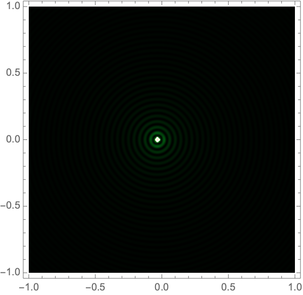
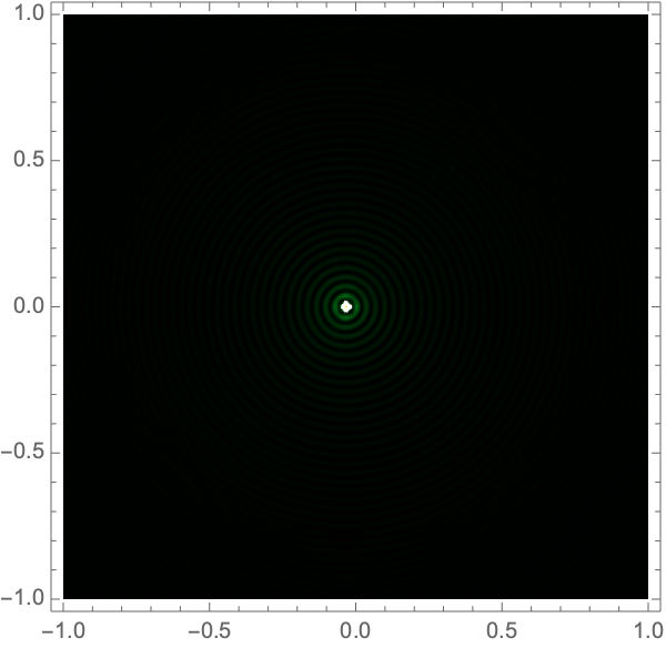
where \({}_1F_1\) is Kummer’s confluent hypergeometric function. Figure 1 shows interference patterns for this case.

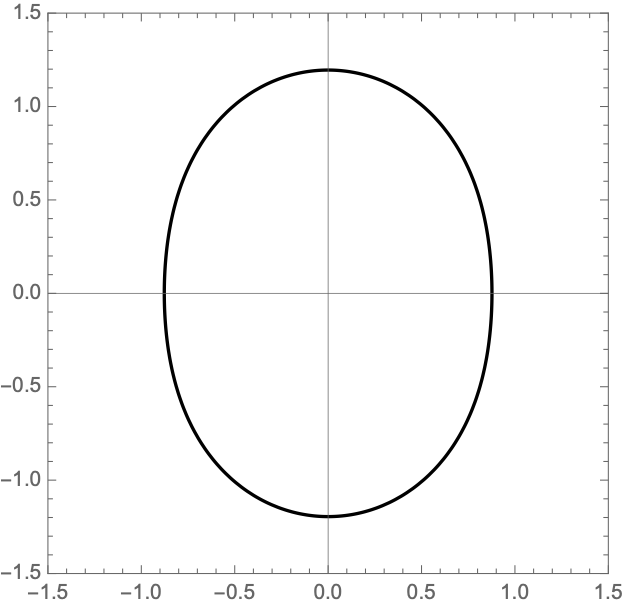
The result is beautifully simple but unrepresentative since a small perturbation of the lensing phase drastically alters the caustics and the consequent interference pattern. As a further step towards realism, we add a shear field:

\[\varphi(\boldsymbol{x}) = - \log x + \frac{1}{2}\gamma (x^2 - y^2),\]

with \(\boldsymbol{x}=(x_1,x_2)\) and a shear strength \(0\leq \gamma \leq 1\) as could, for example, represent the tidal force form an external mass located a distance \(\gamma^{-1/2}\) from the lens. In geometric optics, the single lens with a shear field induces the Lagrangian map,

\[\xi(\boldsymbol{x}) = \left(1-\frac{1}{x}\right) \boldsymbol{x} +\gamma (-x1,x2),\]

sending points from the lens plane to the screen. This map forms a caustic at the critical curve defined by the condition \(\det(\nabla \xi) = 0\),

\[\mathcal{M} =\left \{ r (\cos \theta, \sin \theta) \,\bigg| \,r = \frac{1}{\sqrt{1- \gamma^2}} \sqrt{ \sqrt{1-\gamma^2 \sin^2 2 \theta} -\gamma \cos 2 \theta} \text{ and } \theta \in [0,2\pi)\right\}.\]

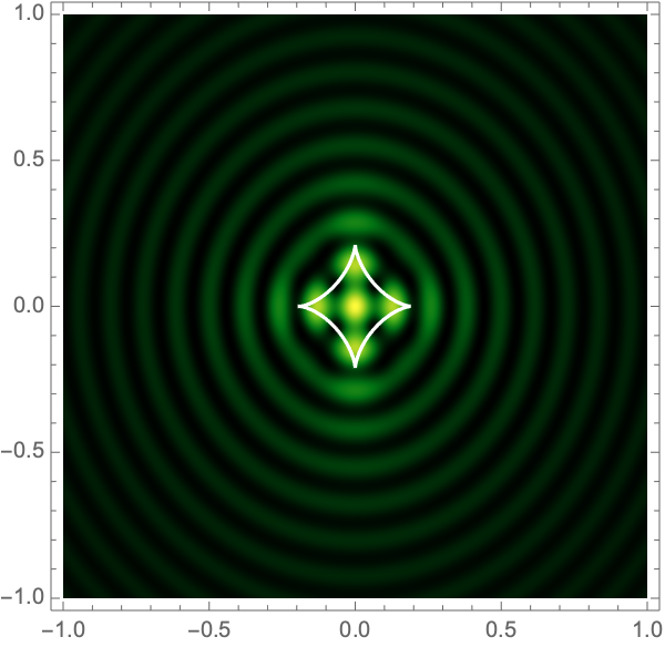
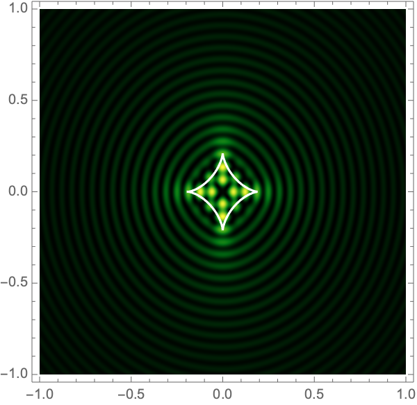
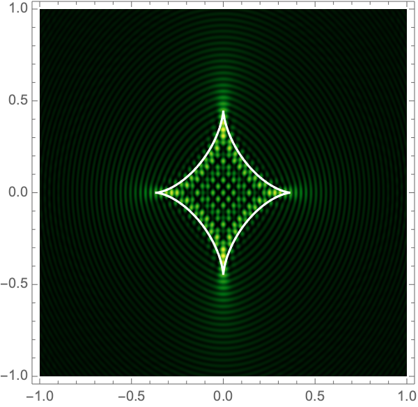
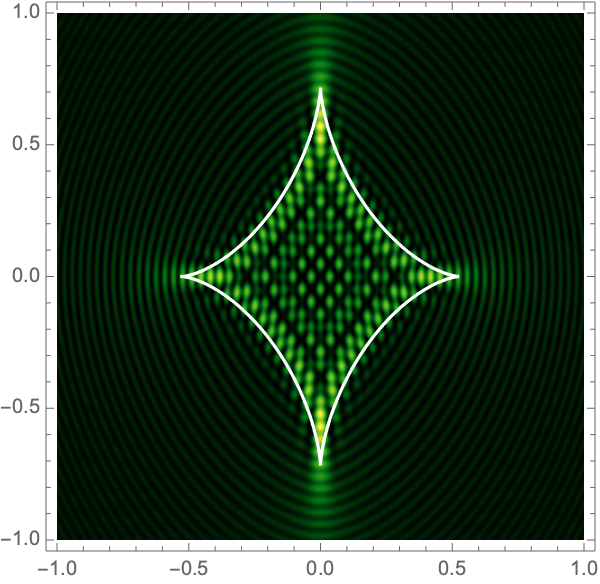
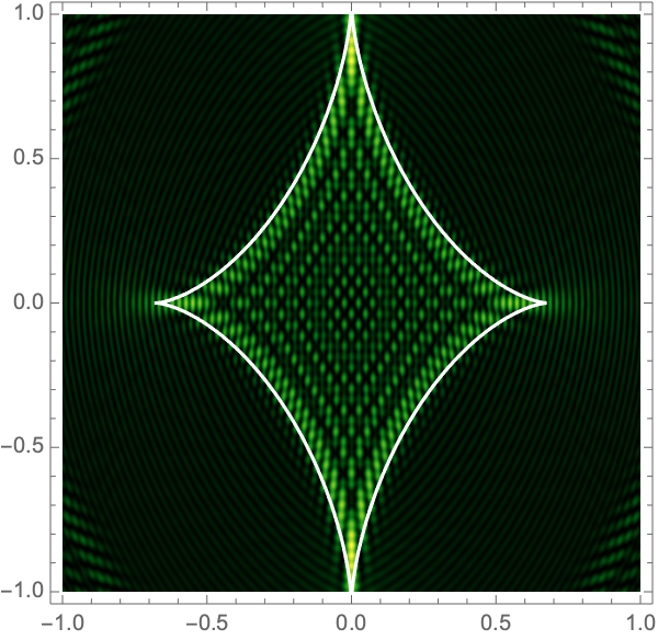
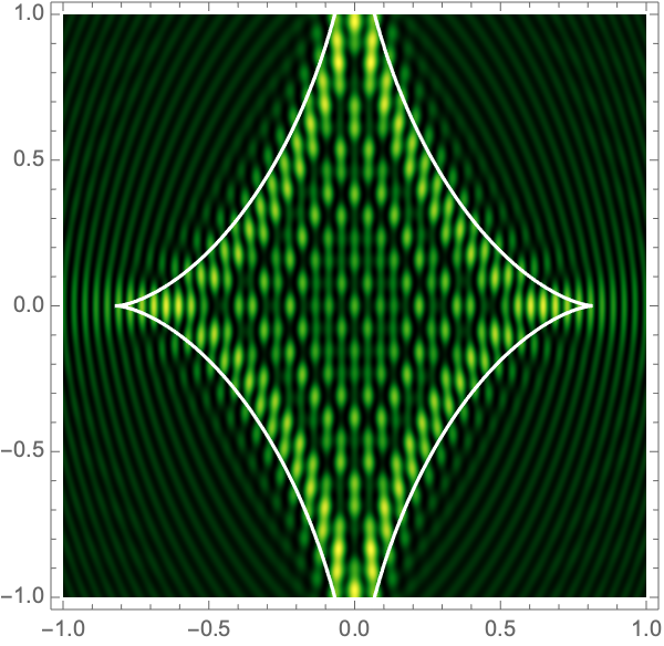
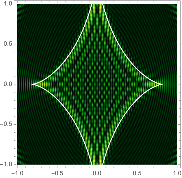
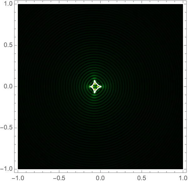
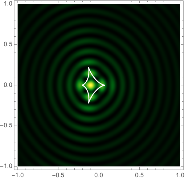
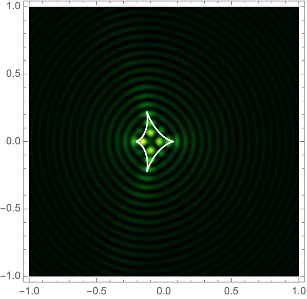
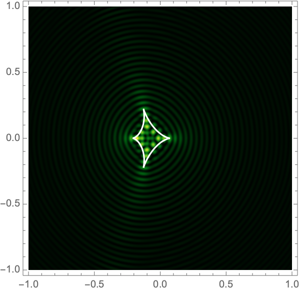
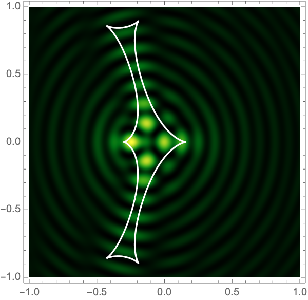
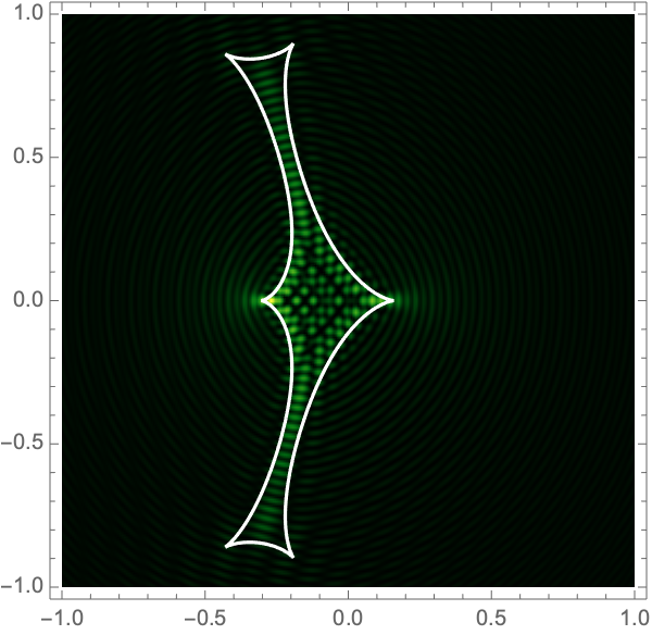
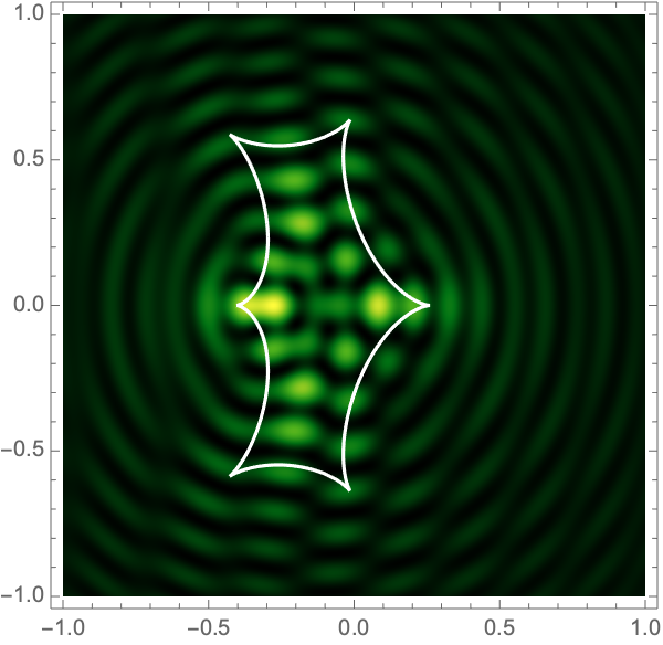
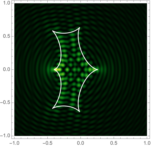
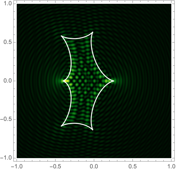
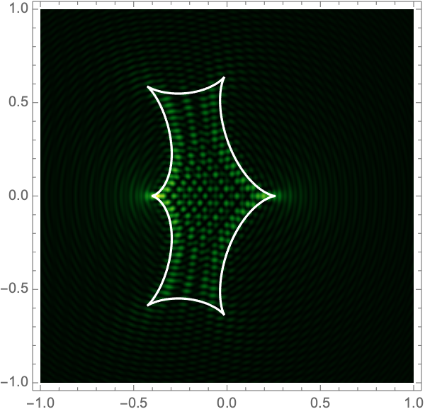
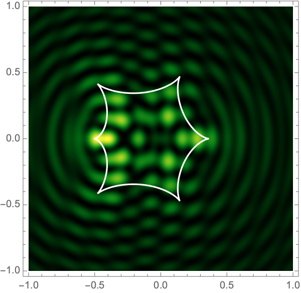
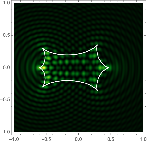
The Lagrangian map takes the critical curve to the caustic curve \(\boldsymbol{\xi}({M})\) consisting of four fold curves running between four cusp points and forming a curved diamond. This diamond is the curve at which the intensity in the geometric optics approximation diverges. The Kirchhoff-Fresnel integral has generically four saddle points, with two or four being real depending on whether \(\boldsymbol{y}\) is outside or inside the caustic curve. The outside and inside of the caustic curve are respectively double- and quadruple-image regions.

To evaluate the lens in wave optics, we use polar coordinates centred at the lens: \(\boldsymbol{x} = r(\cos \theta , \sin \theta )\). In these coordinates, the integrand is an analytic function of the radial and angular coordinates,

\[\psi(\boldsymbol{y}) =\frac{\Omega}{2\pi i} \int_{0}^\infty \int_0^{2\pi} e^{i \Omega \left[ ((r\cos \theta - \mu_x)^2 + (r\sin \theta - \mu_y)^2) / 2 - \log r + \frac{\gamma }{2} r^2(\cos^2\theta - \sin^2\theta) \right]} r \mathrm{d} \theta \mathrm{d} r,\]

with \(\boldsymbol{y} = (y_1,y_2)\). The radial integral is subtle since the integrand oscillates an infinite number of times. We use Picard-Lefschetz theory to perform it, at each value of \(\theta\), defining

\[g_{\theta}(\boldsymbol{y}) = \int_{\mathcal{J}_\theta} e^{i \Omega \left[ {1\over 2}((r\cos \theta - x_1)^2 + (r\sin \theta - x_2)^2) - \log r + {1\over 2} \gamma r^2 \cos 2\theta \right] + \log r} \mathrm{d} r,\]

with the Lefschetz thimble \(\mathcal{J}_\theta\) obtained by a continuous deformation of the original integration domain \((0,\infty)\) into the complex \(r\)-plane (see Fig. 3 for an example). This deformation removes the oscillations from the radial integral.

The remaining integral over \(\theta\)

\[\psi(\boldsymbol{y}) =\frac{\Omega}{2\pi i} \int_0^{2\pi} g_\theta (\boldsymbol{y})\mathrm{d}\theta,\]

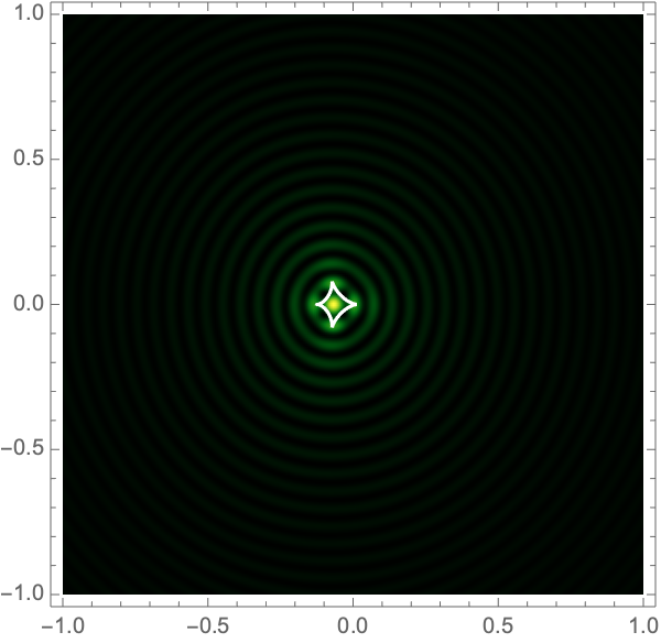
can be evaluated with more traditional numerical methods. See Fig. 4 for the interference patterns of the single gravitational lens with a shear of \(\gamma=0.1-0.5\) for \(\Omega=25-100\).

Binary gravitational lens

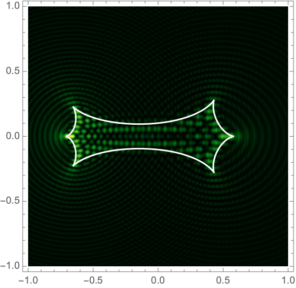
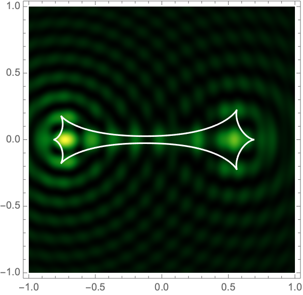
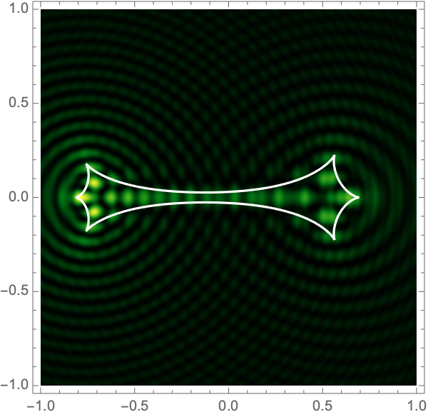
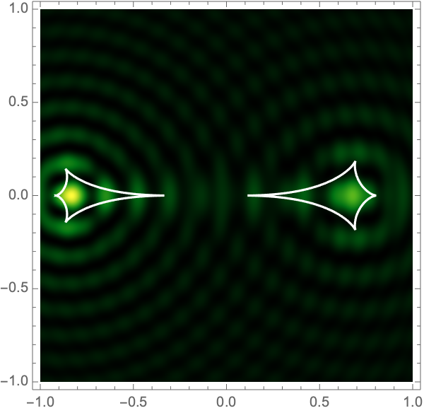
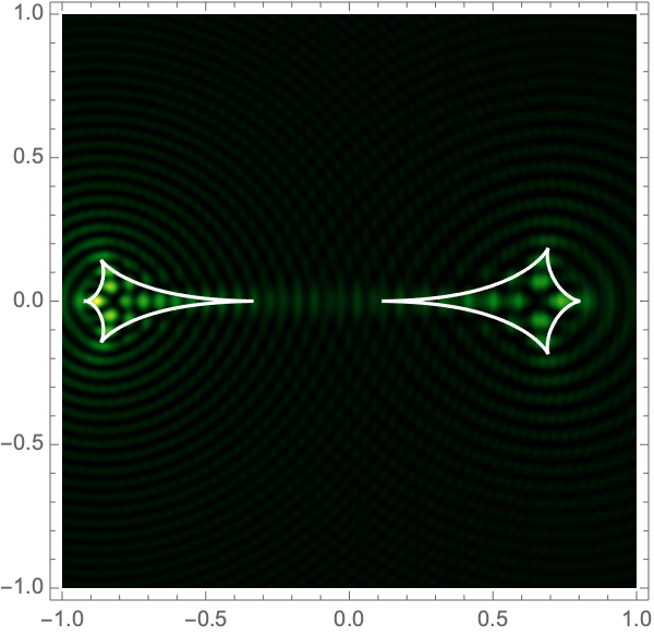
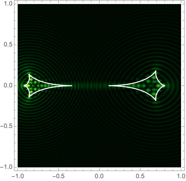
A binary gravitational lens has a lensing phase

\[\varphi(\boldsymbol{x}) = -f_1 \log|\boldsymbol{x} + \boldsymbol{r}| - f_2 \log|\boldsymbol{x} - \boldsymbol{r}|.\]

with \(\boldsymbol{r} = (a,0)\) for some \(a>0\). The Lagrangian map

\[\xi(\boldsymbol{x}) = \left(x_1 - \frac{f_1(x_1+a)}{| \boldsymbol{x} + \boldsymbol{r}|} - \frac{f_2(x_1-a)}{| \boldsymbol{x} - \boldsymbol{r}|}, x_2 - \frac{f_1 x_2}{\| \boldsymbol{x} +\boldsymbol{r}\|} - \frac{f_2 x_2 }{| \boldsymbol{x} - \boldsymbol{2}|}\right)\]

can be used to construct the critical curve, \(\mathcal{M} = \{\boldsymbol{x}| \det \nabla \xi(\boldsymbol{x}) = 0\}\) and the caustic curve, \(\xi(\mathcal{M})\). It is straightforward to show that outside the caustic curve, three images contribute to the intensity. Two of these are mainly lensed by one of the two lenses and the third is lensed by the combined system. Inside the caustic curve is a five-image region.

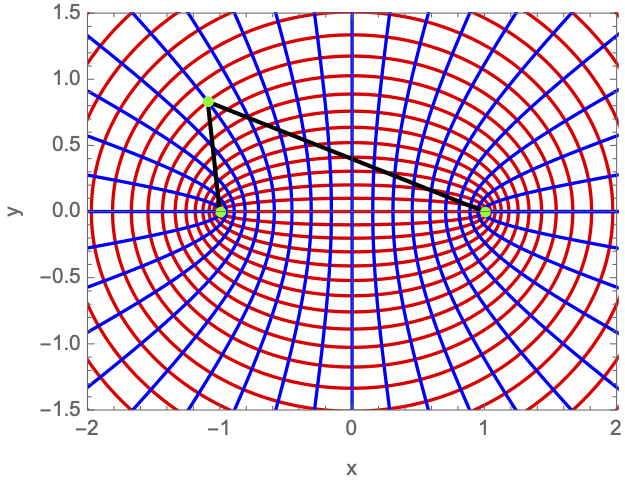
As with the single gravitational lens, it is awkward to apply Picard-Lefschetz methods in Cartesian coordinates since the integrand has branch cuts on the real axis. Instead we use elliptic coordinates, \(\boldsymbol{x}(\tau,\sigma) = a(\cosh \tau \cos \sigma, \sinh \tau \sin \sigma)\), with \(0 < \tau < \infty\) and \(0 < \sigma \leq 2\pi\). Geometrically, these coordinates has two foci at the locations of the two lens masses \(\mp\boldsymbol{r}\). The constant \(\tau\) contours form ovals around the foci (the red curves in Fig. 5). The constant \(\sigma\) contours pass between the two foci (the blue curves in Fig. 5). Note that the variables \(\tau\) and \(\sigma\) are analogous to \(r\) and \(\theta\) in 2d polar coordinates.

In elliptic coordinates, we obtain the identities

\[ \begin{aligned} |\boldsymbol{x} +\boldsymbol{r}\| &= a(\cosh \tau + \cos \sigma),\\ |\boldsymbol{x} - \boldsymbol{r}\| &= a(\cosh \tau - \cos \sigma), \end{aligned}\]

and the Jacobian

\[J(\tau,\sigma) = \frac{a^2}{2} \left( \cosh 2\tau - \cos 2 \sigma\right).\]

Following the calculation for the single gravitational lens, we perform the radial \(\tau\)-integral using Picard-Lefschetz theory

\[g_\sigma(\boldsymbol{y}) = \int_{\mathcal{J}_\sigma} e^{i \Omega \left[ \frac{1}{2}(\boldsymbol{x}(\tau,\sigma) - \boldsymbol{y})^2 - f_1 \log(a(\cosh \tau + \cos \sigma))- f_2 \log(a(\cosh \tau - \cos \sigma))\right] + \log J(\tau,\sigma)}\mathrm{d}\tau.\]

For this integral, it turns out to be most efficient to extend the original integration domain for \(\tau\) to the real line. See Fig. 6 for two examples of the thimble \(\mathcal{J}_\sigma\).

The amplitude is now expressed as an angular integral over a compact domain which we evaluate using conventional integration techniques

\[\psi(\boldsymbol{y}) = \frac{\Omega}{4\pi i} \int_0^{2\pi} g_{\sigma}(\boldsymbol{y}) \mathrm{d}\sigma.\]

Figure 7 shows intensity maps for lens strengths \(f_1=1/3, f_2=2/3\), with separations \(a=0.1-1.0\) and \(\Omega=25-100\).